This is a part of data visualisation practice work created using R including the codes.
Access to data
Synthetic ART-in-HIV data is accessible from https://figshare.com/ndownloader/files/35249488. Below is a brief information about the data loaded.
  # load csv file
   df <- read_csv("https://figshare.com/ndownloader/files/35249488") %>%
   glimpse()
The dataset includes 16 columns and 534,960 observation (rows). All variable types are numeric with decimal points
Data cleaning
Firstly, let’s check if there are missing values in the dataset. Below table shows number of missing value in eash column. After checking, there is no missing value found.
sapply(df, function(x) sum(is.na(x)))
Next, let’s tidy up variable names. We are going to remove space between the variable name and replace with ‘_’, remove ‘()’ as well as replace the first variable name from ‘…1’ to ‘ID’ as below. We created replicated dataset of ‘df’ and named it ‘df1’ and changes were made to ‘df1’ instead of raw dataset. Variable names after the change are as following.
 # copy the dataset before making changes
   df1 <- df

 # replace column names
   colnames(df1) %<>% str_replace_all(c("\\s"= "_", "-"= "_", "\\."="", "\\("="","\\)"="", "1"="ID"))
   colnames(df1)
Then let’s fix variable types. Currently all of the variables are double integer. According to the information provided, variable types are:
Numeric: VL, CD4
Binary: Gender, Extra_pk_En, VL_M, CD4_M, Drug_M
Categorical: Ethnic, Base_Drug_Combo, Comp_INI,Comp_NNRTI,Extra_PI
Integer: ID, PatientID, Timepoints
Updated variable types are listed below.
  df1 <- df1 %>%
    # change selected variables to factor variable
    mutate_at(vars(Gender,Ethnic,Base_Drug_Combo,Comp_INI,Comp_NNRTI,Extra_PI), as.factor) %>%
    # change selected variables to logical variable
    mutate_at(vars(Extra_pk_En,VL_M,CD4_M,Drug_M), as.logical) %>%
    # change selected variables to integer variable
    mutate_at(vars(ID,PatientID, Timepoints), as.integer)

  # check updated variable types
  str(df1)
ID, PatientID and Timepoints variables are integer type, Gender, Ethnic, Base_Drug_Combo,Comp_INI,Comp_NNRTI,Extra_PI are factor type and Extra_pk_En, VL_M, CD4_M, Drug_M are logical type. Notice that Ethnic variable has 3 levels of “2”,”3”,”4” without factor “1”. According to background information “1” is Asian, however there is no data its value is “1”. As there was no missing value therefore we assume that there is was no patient whose ethnicity is Asian for now. However in real case, data might be missing and it will need further check before continuing the analysis.
Data dictionary
Data dictionary is created with label added, and set ID variable as unique identifier variable.
  # add a variable description to label
    df1.labels <- c(ID = "Unique identifier",
                  VL = "Viral Load (copies/mL)",
                  CD4 = "Absolute count for CD4 (cells/μL)",
                  Rel_CD4 = "Relative count for CD4 (cells/μL)",
                  Gender = "Gender. 1 = Male, 2 = Female",
                  Ethnic = "Ethnicity. 1 = Asian, 2 = African, 3 = Caucasian, 4 = Other ",
                  Base_Drug_Combo = "Base drug combination. 0 = FTC + TDF, 1 = 3TC + ABC, 2 = FTC + TAF, 3 = DRV + FTC + TDF, 4 = FTC + RTVB + TDF, 5 = Other",
                  Comp_INI = "Complementary INI. 0 = DTG, 1 = RAL, 2 = EVG, 3 = Not Applied",
                  Comp_NNRTI = "Complementary NNRTI. 0 = NVP, 1 = EFV, 2 = RPV, 3 = Not Applied",
                  Extra_PI = "Extra PI. 0 = DRV, 1 = RTVB, 2 = LPV, 3 = RTV, 4 = ATV, 5 = Not Applied",
                  Extra_pk_En = "Extra pk enhancer. 0 = False, 1 = True",
                  VL_M = "VL measured. 0 = False, 1 = True",
                  CD4_M = "CD4 measured. 0 = False, 1 = True",
                  Drug_M = "Drug recorded. 0 = False, 1 = True",
                  PatientID ="Synthetic patient ID",
                  Timepoints ="Time steps in the time series")

 # create a data dictionary with labes and set variable "ID" as an Identifier variable
   tab <- create_dictionary(df1, id_var="ID",  var_labels = df1.labels)
   knitr::kable(tab, format = "html",table.attr = "style='width:60%;'",position = "center") %>%
   kableExtra::kable_styling()

EDA on univariate variables
Patient demographics
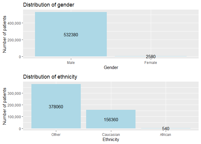
Over 99% are male whereas only less than 1% are female data collected. Majority of patients are other ethnicity that are not Asian, African nor Caucasian following Caucasian and African. There is no Asian patient data collected.
 # barplot of Gender variable
   g <- ggplot(df1, aes(x= Gender)) +
   geom_bar(stat="count", fill="lightblue") +
   stat_count(binwidth = 1,
              geom = 'text',
              aes(label = after_stat(count)),
              position = position_stack(vjust = 0.5)) +
   labs(title = "Distribution of gender",
        x = "Gender",
        y = "Number of patients") +
   scale_x_discrete(breaks=c(1,2),
                   labels=c("Male","Female")) +
   scale_y_continuous(labels = scales::comma)

 # barplot of Ethnic variable
   e <- ggplot(df1, aes(x=forcats::fct_infreq(Ethnic))) +
   geom_bar(stat="count", fill="lightblue") +
   stat_count(binwidth = 1,
              geom = 'text',
              aes(label = after_stat(count)),
              position = position_stack(vjust = 0.5)) +
   labs(title = "Distribution of ethnicity",
        x = "Ethnicity",
        y = "Number of patients") +
   scale_x_discrete(breaks=c(1,2,3,4),
                   labels=c("Asian","African", "Caucasian","Other")) +
   scale_y_continuous(labels = scales::comma)

 # layer plots
   library(gridExtra)
   grid.arrange(g,e,nrow=2)
Health status data measurement
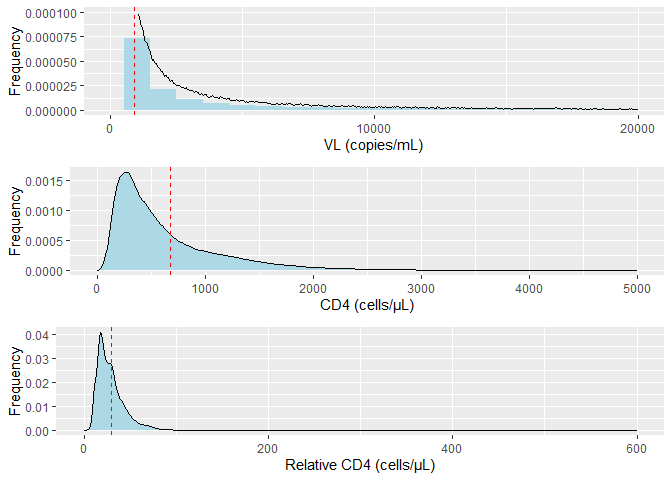
Viral load(VL), absolute count for CV4(CD4) and Relative count for CD4(Rel_CD4) are collected as indicative of the patient’s health status. Each graph shows range of VL, CD4 and Rel_CD4 counted and its average in dashed line.
  v <- ggplot(df1, aes(x = VL)) +
       geom_histogram(fill ="lightblue",binwidth=1000, aes(y=after_stat(density))) +
       geom_density(aes(y=after_stat(density))) +
       scale_x_continuous(breaks=c(0,10000,20000), limits =c(0,20000)) +
       scale_y_continuous(limits=c(0,0.0001), labels = scales::comma) +
       geom_vline(aes(xintercept=mean(VL)),
                  color = "red", linetype="dashed", size=0.3) +
       labs(x = "VL (copies/mL)",y = "Frequency")


  c <- ggplot(df1, aes(x = CD4)) +
       geom_density(fill="lightblue") +
       scale_x_continuous(breaks=c(0,1000,2000,3000,4000,5000), limits =c(0,5000)) +
       geom_vline(aes(xintercept=mean(CD4)),
                 color ="red", linetype="dashed", size=0.3) +
       labs(x = "CD4 (cells/μL)",y = "Frequency")

  r <- ggplot(df1, aes(x = Rel_CD4)) +
       geom_density(fill="lightblue") +
       scale_x_continuous(breaks=c(0,200,400,600), limits=c(0,600)) +
       geom_vline(aes(xintercept=mean(Rel_CD4)),
                     color="red", linetype="dashed", size=0.3) +
       labs(x = "Relative CD4 (cells/μL)",y = "Frequency")

   # layer plots
     grid.arrange(v,c,r, ncol=1, nrow=3)
HIV treatment factors
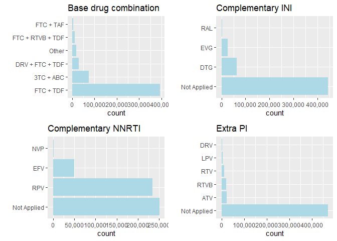
Distribution of base drug combination(Base_Drug_Combo),complementary INI(Comp_INI), complementary NNRTI(Comp_NNRTI) and extra PI(Extra_PI) are described as below.
 # base drug combo distribution
   d <- ggplot(df1,aes(y = fct_infreq(Base_Drug_Combo))) +
        geom_bar(fill="lightblue") +
        labs(title = "Base drug combination",y = "") +
        scale_y_discrete(breaks=c(0,1,2,3,4,5),
                 labels=c("FTC + TDF", "3TC + ABC", "FTC + TAF", "DRV + FTC + TDF", "FTC + RTVB + TDF", "Other")) +
        scale_x_continuous(labels = scales::comma)

 # complementary INI distribution
   i <- ggplot(df1,aes(y = fct_infreq(Comp_INI))) +
   geom_bar(fill="lightblue") +
   labs(title = "Complementary INI",y = "") +
   scale_y_discrete(breaks=c(0,1,2,3),
                    labels=c("DTG", "RAL", "EVG", "Not Applied")) +
   scale_x_continuous(labels = scales::comma)

  # complementary NNRTI distribution
    n <- ggplot(df1,aes(y = fct_infreq(Comp_NNRTI))) +
    geom_bar(fill="lightblue") +
    labs(title = "Complementary NNRTI",y = "") +
    scale_y_discrete(breaks=c(0,1,2,3),
                    labels=c("NVP", "EFV", "RPV", "Not Applied")) +
    scale_x_continuous(labels = scales::comma)

  # Extra PI distribution
    ep <- ggplot(df1,aes(y = fct_infreq(Extra_PI))) +
          geom_bar(fill="lightblue") +
          labs(title = "Extra PI",y = "") +
          scale_y_discrete(breaks=c(0,1,2,3,4,5),
                           labels=c("DRV", "RTVB", "LPV", "RTV", "ATV", "Not Applied")) +
         scale_x_continuous(labels = scales::comma)

   # layer plots
     grid.arrange(d,i,n,ep,ncol=2, nrow=2)
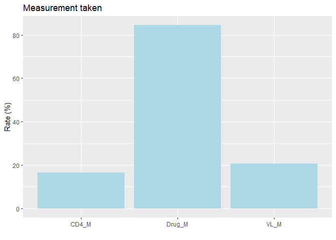
Variables VL_M,CD4_M and Drug_M indicate if the measurement are taken. Following graph depicts rate of each measurement. Drug is taken 84.4%, VL and CD4 are taken 20.7% and 16.7% respectively.
   # plot with VL_M,CD4_M,Drug_M variables
     df1 %>%
           pivot_longer(cols = c("VL_M","CD4_M","Drug_M")) %>%
           group_by(name) %>%
           summarise(frequency_of_1 = mean(value == 1) *100) %>%
           ggplot() +
           aes(name, frequency_of_1) +
           geom_col(fill="lightblue") +
           labs(title = "Measurement taken",x ="", y = "Rate (%)")
—End of document—