All images and statistical results are created by using R.
About the data
Load data
df <- read.csv("Data/contraceptives.csv")

#is.na(df) # no missing value


Statistical summary
summary(df)
##     month              combined          mini
##  Length:48          Min.   :288.8   Min.   :21.00
##  Class :character   1st Qu.:301.8   1st Qu.:22.18
##  Mode  :character   Median :309.2   Median :22.95
##                     Mean   :309.4   Mean   :22.82
##                     3rd Qu.:316.3   3rd Qu.:23.52
##                     Max.   :331.7   Max.   :24.60
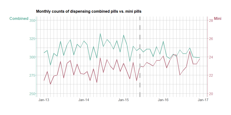
Fig 1.1 Monthly dispensing of PBS-subsidised combined and mini pills per 10,000 women of reproductive age between January 2013 and December 2016
During observation time, combined pills are dispensed between 288.8 to 331.7 times, and 21 to 24.6 times of mini pills are dispensed during the same time. Use of mini pills are clearly increased from 2013 to 2017 whereas combined pills do not show strong trend of increase or decrease.
Time series data analysis
From the raw data, we created a time series data starting from January 2013 to December 2016 by monthly basis. We will examine its trend (Stationarity), autocorrelation and seasonality.
- Stationarity
As illustrated in fig 1.1 we can see that there is no obvious increase or decrease trend in combined pills data over the time. In fig 1.3, stationarity of mini pills are removed in log difference form, however as our interest is an effect on combined pills, and mini pills are considered as a control variable in this study, we will use raw form of data instead of log form. We can also see there is annual cycle in combined pills in fig 1.2 and fig 1.3 which will be examined for seasonality.
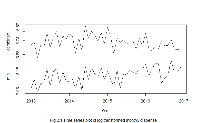
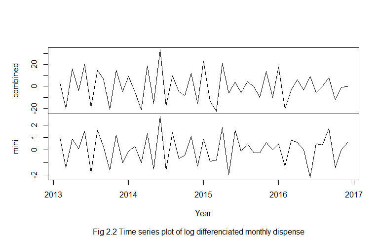
Also, Augmented Dickey-Fuller (ADF) test is conducted for a statistical check. Hypothesis of ADF test is H0: time series is non-stationary (p > 0.05), H1: time series is stationary (p ≤ 0.05)
##
##  Augmented Dickey-Fuller Test
##
## data:  ts_c
## Dickey-Fuller = -3.6574, Lag order = 3, p-value = 0.03812
## alternative hypothesis: stationary
From ADF test, p-value of combined pill is 0.038. Thus, we take the alternative hypothesis, considering the time series is stationary.
- Seasonality
Fig 2.3 shows the counts of combine pills dispensed in each year. There is a clear seasonal trend, the number of dispensing combine pills is drastically jumps in January and from December, and drops largely towards March. Then it starts increase from March to June. Decomposed seasonal plot fig 2.4 supports yearly trend in the data where the number of dispense hits the bottom in early year, then increasing through rest of the year.
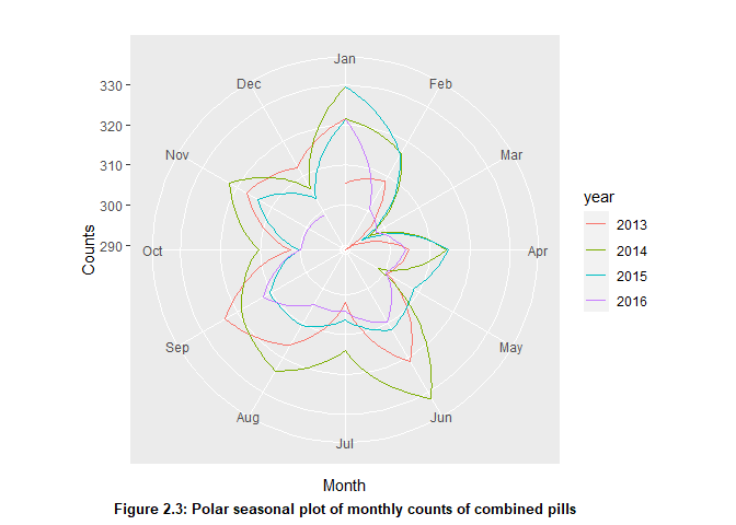
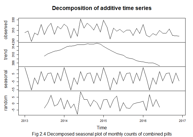
Below is Kruskall Wallis test result for the seasonality test. Hypothesis of the test is H0: all months have the same mean, therefore the data is no seasonality (p > 0.05), H1: time series has a seasonality (p ≤ 0.05)
## Test used:  Kruskall Wallis
##
## Test statistic:  36.07
## P-value:  0.0001646953
P-value of the test is less than 0.05 which indicates there is a seasonality in the data.
In Australia, the PBS subsidises medicines, leading to a yearly pattern in medicine dispensing claims. Once individuals or families hit the “Safety Net threshold” in a year, their co-payments are reduced, incentivising them to refill prescriptions more frequently towards year-end. This results in a surge in prescriptions in December, followed by a drop in January(Schaffer et al., 2021). The seasonality of combined pills counts also following similar pattern due to the PBS safety net threshold system.
- Autocorrelation
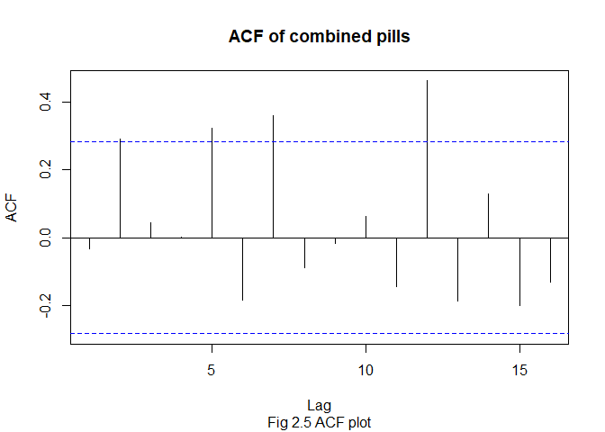
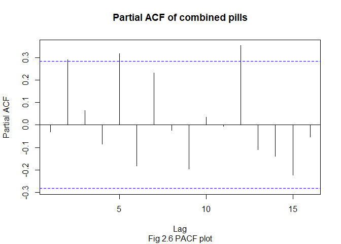
Following plots are ACF, PACF and CCF against mini pills. ACF and PACF interpret delayed impact of combine pills only, and we included mini pills in CCF as an external regression.
##
## Autocorrelations of series 'X', by lag
##
##    -13    -12    -11    -10     -9     -8     -7     -6     -5     -4     -3
## -0.094  0.386 -0.007  0.148 -0.035 -0.136  0.041 -0.337 -0.031 -0.167 -0.082
##     -2     -1      0      1      2      3      4      5      6      7      8
##  0.119 -0.374  0.426 -0.252  0.054 -0.170 -0.208  0.014 -0.429 -0.095 -0.385
##      9     10     11     12     13
## -0.170 -0.073 -0.291  0.183 -0.223
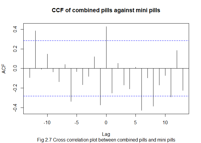
In fig 2.5 and 2.6, ACF and PACF shows several peaks then drastic drop in next a few sequence. This probably indicates its seasonality as discovered above. The cross correlation at lag -12 and 0 is 0.386 and 0.426 respectively. From fig 2.7, most of the time the correlation between combined pills are mini pills are negative that tells the number of dispensing combined pills decrease when more mini pills are dispensed as observed in the raw data as well.
Most of peak values in the plots are out of 95% confidence interval but very close, we will conduct statistical test to ensure the delayed impact. Since Ljung-box test can examine one variable at a time, Ljung and Box Portmanteau test was used as the fucntions of BoxPierce and LjungBox are more accurate than Box.test function and can be used in the univariate or multivariate time series at vector of different lag values as well as they can be applied on an output object from a fitted model described in the description of the function BoxPierce. Hypotheses of the test are, H0: there is no auto/ cross correlation in time series (p > 0.05) and H1: there is an auto/cross correlation in time series (p ≤ 0.05).
##  lags statistic df      p-value
##    10  125.2702 40 1.012246e-10
P-value of the test less than 0.05, therefore we reject Null hypothesis and consider that there is a delayed impact in the time series.